This power subsystem is designed for a solar‑powered, battery‑backed IoT node used in agricultural monitoring and remote sensing. The node must keep a microcontroller (MCU) and essential logic alive 24/7 from a continuous 3.3 V rail, while switchable auxiliary rails (12 V, 5 V, 3.3 V_AUX) power sensors, radios, and actuators only when needed via a common EN_AUX signal. The design must tolerate a harsh outdoor environment (temperature swings, moisture, dirt, ESD), handle panel voltages up to the high‑20 V range typical of “12 V‑class” PV modules, and protect the Li‑ion battery pack from abuse (over/under‑voltage and current events) with detailed state‑of‑charge visibility.
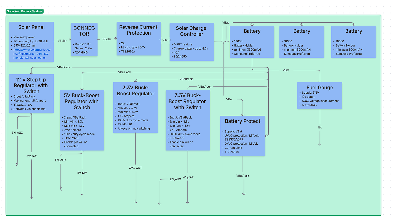
At a high level (see the provided block diagram), energy flows from a rugged Deutsch DT solar connector into reverse‑current protection and an MPPT solar charger, then into a 1‑cell 18650 battery pack (cells in parallel for capacity). Downstream of the pack, a protect eFuse enforces UVLO/OVLO and current limiting. One always‑on 3.3 V buck‑boost regulator feeds the MCU (“3V3_CNT”). Three auxiliary regulators (12 V step‑up, 5 V buck‑boost, 3.3 V buck‑boost) are gated by EN_AUX to minimize idle draw. A fuel‑gauge IC reports SoC and voltage to the MCU over I²C.
Design decisions are justified below with alternatives and trade‑offs. Each section ends with a concise comparison table. Inline numeric citations use APA‑style bracket numbering (e.g., [4]); the full references list appears at the end.
2) Solar input and front‑end
2.1 PV panel and field connector
What we used and why. The system expects a “12 V‑class” PV module (≈17–18 V at maximum power, ≈21–22 V open‑circuit, depending on temperature) connected through a Deutsch DT‑series 2‑pin sealed connector. DT connectors are widely used in agricultural and off‑highway equipment for their IP‑rated seals, latch robustness, and vibration resistance, reducing water ingress and intermittent contact risks that plague generic DC barrel jacks in the field [14]. The higher Voc of “12 V” panels is normal and ensures headroom for charging; this is handled by the downstream MPPT charger [20]. RS ComponentsAltE Store
Alternatives considered. M8 circular connectors (industrial sensors), and unsealed barrel jacks. DT won for sealing and tactile locking; M8s are excellent but require panel‑mount bulkheads and are costlier; barrel jacks were rejected for poor ingress protection.
Option
IP/Sealing
Current rating
Field serviceability
Typical cost
Notes
Deutsch DT‑2 (chosen)
IP67/68 with seals
~13 A per size‑16 contact
Crimp contacts, positive latch
$$
Proven in ag/off‑road [14]
M8 A‑coded
IP67/68
3–4 A typical
Threaded; panel‑mount bulkhead
$$$
Great, but higher BoM and assembly cost
DC barrel jack
Poor
1–5 A
Easy
$
Not weatherproof—unsuitable outdoors
2.2 Reverse‑current and surge protection (PV side)
What we used and why. A high‑voltage eFuse with reverse‑polarity/ reverse‑current blocking (TI TPS2660x family) protects the system from wiring mistakes and prevents the battery from back‑feeding a dark panel. Compared with a Schottky diode, the eFuse avoids large conduction losses, supports adjustable current limit, and tolerates the ≈30 V worst‑case Voc/ transients from “12 V” panels [3]. Texas Instruments
Alternatives considered.
Option
Conduction loss
Reverse blocking
Accuracy/features
Complexity
Suitability
eFuse TPS2660x (chosen)
Low (MOSFET)
Yes (OVP, RCP)
OVP/UVP/ILIM, telemetry (varies)
Medium
Best overall protection to 60 V [3]
Ideal‑diode controller (LTC4412, LM5050‑1)
Very low
Yes
No current limit; add parts for OVP
Medium
Efficient, but less comprehensive [8][9]
Schottky diode
High
Partially
None
Low
Simpler; unacceptable power loss at >1–2 A
Rationale: In a remote node, survivability beats small BoM savings. The eFuse gives correct behavior under miswiring, hot‑plug, and panel brownouts.
2.3 MPPT solar charge controller
What we used and why.TI bq24650—a synchronous buck charger with integrated constant‑voltage MPPT loop. It reduces charge current so the panel operates near its programmed MPP and supports a wide PV input range, ideal for “12 V‑class” modules [4]. The device handles pre‑charge, termination, and status; it charges a 1‑cell Li‑ion pack to 4.2 V (adjustable via feedback). Texas InstrumentsFarnell
Alternatives considered.
IC
Topology
Input range
MPPT method
Max I_CHG
Notes
bq24650 (chosen)
Buck, ext. FETs
5–28 V (typ)
Constant‑voltage input regulation
5 A‑class (design‑dependent)
Well‑documented PV tracking [4]
ADI LT3652
Monolithic buck
4.95–32 V
Input‑voltage regulation (peak power tracking)
Up to 2 A
Excellent for compact, moderate‑current designs [12]
CN3791
Buck controller
4.5–28 V
MPPT (1.205 V ref)
Up to 4 A
Cost‑effective; fewer protections [13]
MCP73871
Linear
3.5–6 V
None (power‑path mgr)
~1 A
Good for USB/small PV; poor efficiency at high Vin [11]
Rationale: The bq24650 offers the best balance of input range, efficiency, and documented MPPT behavior for our panel class. If the system prioritized minimal BoM over peak charge current, LT3652 would be a credible alternative. Analog Devices
Battery longevity note. If lifetime cycling is paramount, the charge voltage can be reduced (e.g., 4.10 V) to extend cycle life at the cost of capacity; industry literature consistently reports large cycle‑life gains when charging below 4.2 V [6]. We keep 4.20 V here to preserve full capacity for high‑peak loads, with the option to derate later via the feedback divider. Battery University
3) Energy storage: 1‑cell 18650 battery pack
What we used and why. A 1S (single‑cell) Li‑ion pack built from multiple 18650 cells in parallel to increase capacity and peak current while keeping the system at 3.0–4.2 V. This keeps downstream converters efficient and allows a single charger IC. Using reputable cells (e.g., Samsung 30Q/35E) ensures consistent impedance and cycle life, important for cold starts and radio bursts. Typical capacities are 3000–3500 mAh per cell (exact choice is a BoM decision). For long life in duty‑cycled applications, we avoid deep discharge (see UVLO in §3) and, if needed, can adopt a lower float voltage per note above [6].
Alternatives considered. 2S Li‑ion (higher bus simplifies 12 V boost but increases parts count), or LiFePO₄ 1S (safer/higher cycle life but lower energy density, different charger). We chose 1S Li‑ion to minimize IC diversity and maintain high converter efficiency at light loads.
4) Battery‑side protection (eFuse + supervisors)
What we used and why. A battery‑side eFuse (TI TPS25946) provides adjustable current limiting, UVLO and OVLO, inrush control, and reverse‑current control. This device cleanly disconnects the pack from downstream rails on faults (shorts, over‑voltage), limiting stress and preventing latch‑ups when loads hot‑plug. A dedicated voltage supervisor provides precise UVLO around 3.3 V (to preserve cell health) and OVLO around 4.1 V (optionally used if we choose to limit the system bus during charge handover). The eFuse’s integrated FET and control loop are significantly more predictable than polymer fuses + discrete MOSFETs in low‑power electronics [7]. Texas Instruments
Alternatives considered.
Option
Pros
Cons
Suitability
eFuse TPS25946 (chosen)
ILIM/OVLO/UVLO, inrush control, reverse current features
Adds IC cost; layout care
Robust, tunable protection [7]
Pack‑level protector (DW01A + MOSFETs)
Very low cost, ubiquitous
Fixed thresholds, no current telemetry or ramp
OK for consumer packs; limited system control [18]
“Rely on charger limits only”
Minimal BoM
No downstream short protection; risky in field
Not acceptable
5) System rails, enables, and power‑gating
A single always‑on 3.3 V rail powers the MCU and fuel gauge. Aux rails (12 V, 5 V, 3.3 V_AUX) are disabled by default and only enabled when tasks require them. This power‑gating strategy slashes idle draw by removing both regulator quiescent current and sensor leakage when not in use. Where loads have large input capacitance (e.g., radios, solenoids), the enable sequence lets the eFuse and regulator soft‑starts tame inrush. If particularly aggressive inrush control is required per load, a small load switch (e.g., TPS22965) at the rail point‑of‑load can add extra slew‑rate control with microamp IQ [17]. Texas Instruments
5.1 Always‑on 3.3 V (MCU rail): synchronous buck‑boost (TPS63020)
What we used and why. The TPS63020 maintains 3.3 V across the full battery span (≈3.0–4.2 V), seamlessly transitioning between buck and boost. Its 100% duty‑cycle mode minimizes switching losses and ripple when Vin is only slightly above Vout (common at 3.5–3.8 V), which is ideal for a quiet MCU rail. It offers solid light‑load efficiency without the dropout problems a buck‑only would have near 3.3 V [1]. Texas Instruments
Key alternatives (and when they might win).
Option
Efficiency across 3.0–4.2 V
IQ (typ.)
EMI/noise
Notes
Buck‑boost TPS63020 (chosen)
High and flat (buck↔boost)
Low
Good; 100% duty in buck
Best regulation at all SoC [1]
LDO (e.g., TPS7A02)
Drops as Vin↑; worst at 4.2 V
Ultra‑low
Excellent
Great if load is ultra‑low and noise is critical; but loses >20% at 4.2→3.3 V [15]
Buck‑only (TPS62130)
High if Vin≫Vout
Low
Good
Fails as Vin approaches 3.3 V (dropout) [11]
Why we chose buck‑boost: We need guaranteed 3.3 V at any SoC with good efficiency and low ripple for the MCU and I²C devices.
5.2 5 V auxiliary rail: synchronous buck‑boost (TPS63020)
This rail powers 5 V peripherals when EN_AUX is asserted. The topology and IC are intentionally the same as §4.1 to reduce BoM diversity and reuse layout know‑how. Here the converter operates exclusively in boost region (since 3.0–4.2 V → 5 V). A boost‑only converter (e.g., TPS61023) is a valid alternative and can be slightly cheaper with very low IQ, but reusing TPS63020 simplified qualification and thermal modeling [10]. No need to repeat the electromagnetic/compensation discussion already covered in §4.1. Texas Instruments
Targeted differences vs §4.1: • Heavier burst loads expected (USB‑class sensors, analog front‑ends), so we size the inductor and output caps accordingly. • Since the rail is off most of the time, its shutdown IQ dominates—TPS63020’s disable current is sufficiently low for our budget [1].
Focused comparison for 5 V:
Option
Vout
Notes
TPS63020 (chosen)
5 V
Reuse; strong transient handling [1]
TPS61023
5 V
Simpler boost‑only; excellent light‑load IQ [10]
5.3 12 V auxiliary rail: synchronous boost (TPS61377)
What we used and why. The TPS61377 delivers 12 V (and higher) from the 1S bus with 6 A peak switch current capability and ~70 µA IQ; it is well‑suited to solenoids, valves, and instrumentation that need 12 V only intermittently. It supports selectable PFM/PWM for light‑load efficiency, and has OVP/OCP protections. In our design, its enable is tied to EN_AUX [2]. Texas InstrumentsMouser Electronics
Alternatives considered.
Option
Topology
Pros
Cons
Suitability
TPS61377 (chosen)
Boost
High output power, low IQ, compact
Needs careful layout
Best balance for 12–24 V rails [2]
SEPIC controller (LT3757 / LM3478)
SEPIC/Boost
Very wide Vin–Vout, can step‑up/down
External FETs; larger BoM
Overkill here; shines with wide input [16]
Buck‑boost module
Integrated
Fast to implement
Cost/size
Valid for prototypes only
6) Fuel gauging and telemetry
What we used and why.MAX17043 fuel gauge with the vendor’s ModelGauge algorithm. It reports state‑of‑charge and cell voltage over I²C without a sense resistor, minimizing losses and simplifying layout. Its quick‑start and alert thresholds make it easy to implement robust low‑battery behaviors on the MCU [5]. Analog Devices
Alternatives considered.
IC
Sense resistor
Algorithm
Notes
MAX17043 (chosen)
No
Model‑based SoC
Simple integration, low overhead [5]
bq27441
Yes
Impedance‑track CC
High accuracy over aging; more setup [3rd‑party literature, typical]
MAX17048
No
ModelGauge m3
Newer family; similar use case
Why we chose MAX17043: We needed detailed monitoring with minimal BoM/firmware overhead and no shunt losses—ideal for an energy‑constrained node.
7) System integration notes
EN_AUX power domaining. The MCU keeps 3V3_CNT always on. When tasks require peripherals, it asserts EN_AUX. The three auxiliary regulators share EN_AUX, but time‑staggered enables can be added in firmware if inrush events brown the bus. Load‑switches (TPS22965) can be added at individual loads that still need slew‑rate control [17]. Texas Instruments
Grounding and layout. Keep PV return, charger power ground, and switching regulators on a low‑impedance ground plane. Star the eFuse/battery return into that plane to avoid sense errors in the charger/current‑limit network.
Brown‑in/out behavior. The battery‑side eFuse’s UVLO prevents deep discharge; the MPPT charger restarts charging when PV recovers. This coordination avoids “charge‑while‑brown‑out” loops.
Charging set‑points. Default 4.20 V target; optional 4.10 V profile for life extension per §1.3 if a future firmware/BoM revision trades capacity for cycle life [6].
PV voltage expectations. “12 V‑class” panels measuring ≈22 V open‑circuit are normal; the charger’s input regulation (MPPT) is designed for exactly that regime [4][20]. Texas InstrumentsAltE Store
8) Risk assessment and mitigations
Reverse feed and miswiring: eFuse (PV side and battery side) with reverse‑current blocking and OVP/UVP drastically lowers field‑failure risk compared with diodes/polyswitches alone [3][7]. Texas Instruments+1
Battery stress: UVLO around 3.3 V and thermal/OVLO coordination protect cell health. Use matched cells, keep pack impedance low, and configure charger timers appropriately.
EMI/noise on MCU rail: TPS63020’s 100% duty cycle mode and proper LC selection keep ripple low in buck region; place the inductor and input/output caps per datasheet layout guidance [1]. Texas Instruments
Auxiliary burst loads: For solenoids/valves powered by 12 V, include local TVS and flyback paths if inductive; rely on the boost converter’s OCP and the battery‑side eFuse current limit for fault containment [2][7]. Texas Instruments+1
9) Component‑by‑component summaries with alternatives
Below, each block lists only incremental details if it reuses concepts already covered. This avoids repetition and focuses on the differences that matter.
Alternative:TPS61023 (boost‑only) if BoM reduction outweighs reuse [10]. Texas Instruments
9.8 12 V auxiliary
Chosen:TPS61377 boost.
Alternative:LT3757/LM3478 SEPIC for very wide input or higher outputs [16]. Texas InstrumentsOctopart
9.9 Fuel gauge
Chosen:MAX17043.
Alternatives:bq27441, MAX17048.
Why: No shunt, low overhead, simple I²C integration [5]. Analog Devices
10) Verification checklist
PV side • With panel connected and battery absent, confirm eFuse permits forward conduction and bq24650 regulates the input near MPP under load. • In darkness, verify no reverse current into panel (mA‑level leakage only).
Charge parameters • Measure pre‑charge, fast charge, and CV termination currents per design set‑points. • Confirm thermistor (if used) limits charge in cold/hot conditions (bq24650 feature set).
Battery protect • Sweep bus from 2.8 V→3.6 V and confirm UVLO trip around 3.3 V; verify OVLO behavior during charge handover transients. • Short the 5 V/12 V rail at the board edge with a current‑limited supply upstream; confirm eFuse current limit and auto‑retry behavior.
Rails and enables • With EN_AUX low, measure sleep current (goal: dominated by MCU + 3V3_CNT regulator IQ). • Toggle EN_AUX while logging battery current; ensure inrush stays within limits and MCU rail does not dip.
This architecture achieves robust outdoor operation with fine‑grained power control. The bq24650 MPPT stage maximizes energy harvest from “12 V‑class” panels; a 1S Li‑ion pack simplifies conversion stages and maintains efficiency; an eFuse‑centric protection strategy hardens the node against wiring and load faults; and EN_AUX‑gated rails ensure auxiliary loads do not erode standby life. The selected parts strike a practical balance between efficiency, cost, and resilience, and each block has clear alternatives should future requirements shift.
Imagine you are standing at the mouth of a dense jungle, machete in hand. You can hear there might be treasure beyond the vines—rumours of grateful customers, glowing investor slide decks, maybe even the mythical Series B. But you can also sense there are mud pits and hungry bugs waiting to nibble away at your runway. Chapter 0 is where you decide whether the treasure hunt is worth hacking a path at all. Rookie product managers often skip this step (“Let’s just start sprinting!”). Don’t. A disciplined Concept & Feasibility sprint saves you months of rework, melts away the fog of wishful thinking, and gives your team a rallying‑cry they can carry through the inevitable long nights of debugging firmware at 2 a.m.
0.1 Why does this chapter matter so much?
Because every downstream Gantt bar, Jira ticket, and purchase order inherits its reason for existing from the decision you make here. If you launch into schematic capture or mobile‑app wire‑framing without a clear, evidence‑based “Why”, you are basically renting a bulldozer before you know whether you need a flower bed or a skyscraper. Worse, rookie PMs who skip feasibility will end up pitching hazy dreams to stakeholders: “It’s like a Fitbit, but for cats, and also it mines cryptocurrency!” Great, but try defending that budget request in front of Finance once they ask about the cost of Bluetooth mesh on a collar that Fluffy loves to chew.
0.2 The four conversations you must have
1. Pain‑point interview
Find an actual human (or several) who experiences the problem daily. Listen more than you talk. If they don’t use salty language or sigh heavily when describing the pain, the problem probably isn’t acute enough to justify a hardware start‑up’s burn rate.
Example: A facilities manager confesses they lose thousands of euros a month because nobody notices when the industrial freezer starts drifting above –15 °C at 3 a.m.
2. Vision statement
Distill what you heard into one sentence that can fit on a coffee mug. “We give facilities managers Jedi‑like foresight into equipment failures—before the ice‑cream melts.” If the sentence feels flabby or tries to please everyone, keep whittling.
3. High‑level user journey
Plot a simple storyboard: the manager receives a push notification, taps to open a trend graph, dispatches maintenance, and munches a celebratory cinnamon bun because catastrophe was averted. No UI pixel‑pushing yet—think comic strip, not Marvel mock‑ups.
4. Market sanity check
Open a spreadsheet (yes, that dreaded blank grid) and answer: How often does this pain occur? How many people have it? What would each pay for relief? Industry reports, competitor SKU prices on Digi‑Key, and a quick LinkedIn search of how many “Facilities Manager” job titles exist in your target region will get you within respectable accuracy. Rookie PMs worry about decimal places; veterans worry about orders of magnitude.
0.3 Rapid‑fire feasibility experiments
Hardware development can feel glacial, but you can still generate convincing evidence in days:
Range smoke test – Grab an off‑the‑shelf BLE dev‑kit, stick it inside a stainless‑steel freezer, ping it from the corridor, measure RSSI. If signal dies at two metres, you just dodged a connectivity bullet before ordering custom PCBs.
Sensor truthiness check – Borrow a calibrated temperature probe, tape it beside your candidate digital sensor, and record 12 hours of data. Does the cheap sensor drift 3 °C every time the compressor kicks in? Scrap it early.
Stakeholder demo – Pipe the dev‑kit’s data into a free cloud dashboard (ThinkSpeak, Adafruit IO) and show your facilities manager. If they ask, “Can I buy this tomorrow?” you’re onto something. If they shrug, refine or pivot.
Three‑frame storyboard – Identify trigger, action, and outcome. Sketchy is fine; phone photos of sticky notes count.
TAM/SAM/SOM table – Total, Serviceable, Obtainable market estimates. Ten rows is plenty. Include your confidence score and citation links.
Feasibility sprint memo – One page: Hypothesis → Experiment → Data → Verdict → Next step. Readable in three minutes by your VP.
These artefacts are not management‑crust for the sake of ceremony. They act like alignment beacons: when marketing wants to chase another persona or engineering proposes an exotic mmWave radio, you can wave the one‑pager and ask, “Does this serve our freezer‑saving facilities manager story?”
0.5 Cost of skipping
Still tempted to declare “build it and they will come”? Here’s a back‑of‑envelope cautionary tale. A team I mentored spent €60 000 on PCB spins before realising hospitals— their target market—don’t allow 2.4 GHz radios in MRI suites. A two‑hour Feasibility smoke test with a borrowed spectrum analyser would have saved eight months and an engineer’s resignation.
0.6 Building the Go/No‑Go ritual
Humans, especially engineers fuelled by the thrill of blinking LEDs, hate saying “No.” Institutionalise it. Put a calendar invite for a Feasibility Review exactly two weeks after project kickoff. Invite one person each from business, engineering, quality, and customer success. Present your four artefacts, demo any quick prototypes, and end the meeting with a forced vote: Go or No‑Go (pivot counts as No‑Go). Majority rules. Record the decision in your wiki with a timestamp and list of attendees. Future‑you will thank past‑you when auditors or investors ask, “Why did you bet the farm on LoRa rather than NB‑IoT?”
0.7 Common rookie pitfalls and how to dodge them
Pitfall
Why it stings
Antidote
Solution first, problem later – Falling in love with cool tech
You end up hunting for a market
Write your pain statement before touching dev‑kit firmware
Analysis paralysis – Weeks of spreadsheets
Momentum dies, morale dips
Time‑box every research task to days; share imperfect numbers openly
Asking leading questions – “Wouldn’t you love a freezer cloud?”
Users say yes to be polite → False validation
Ask about today’s workaround cost; watch for real emotion
Ignoring hidden constraints – Regulatory bans, building codes
Surprise redesigns cost millions
Phone one industry veteran; ask “What blindsided you last time?”
0.8 Mini case study: The One‑Week Smart‑Freezer Sprint
Monday: Two PMs interview three facility managers, confirm freezer spoilage costs €10 k per incident. Tuesday: Hardware lead slaps a $12 I²C temperature sensor onto a Wio‑Link dev board, streams JSON to Adafruit IO. Wednesday: Cloud intern builds a Grafana panel and SMS alert via Twilio. Thursday: PMs push a demo video to stakeholders; CFO blurts “If this works, we’ll save €1 m annually across all sites.” Friday: Feasibility Review votes Go, but mandates verifying cellular back‑haul where Wi‑Fi is flaky.
Total spend: €300 on parts and pizza. Clarity gained: priceless.
0.9 The Chapter 0 Checklist (print, annotate, stick above your monitor)
Problem statement captured in one brutally short sentence.
At least one interview with a sufferer of the problem, quotes recorded verbatim.
Two‑to‑three user‑journey sketches photographed and uploaded.
Initial market sanity numbers in a spreadsheet, tagged with source links.
One feasibility experiment run, data charted.
Calendar‑blocking for the Go/No‑Go review done; neutral referee invited.
Decision recorded, link pasted into the root of your project repository.
If Go → high‑level risks & next chapter owner assigned.
If No‑Go → a thank‑you note sent to the team; lessons learned documented.
Tape this checklist to your laptop lid. The next time you’re tempted to sprint ahead because “The PCB house has a sale that ends tonight,” glance at box #1. If you can’t recite the problem statement in five seconds, you’re not ready to order copper.
0.10 Wrapping up
Concept & Feasibility is the smallest chapter by calendar time—but the loudest in impact. Treat it like the prologue to your favourite fantasy novel: skip it and the rest of the plot feels confusing and hollow. Invest a focused burst of energy here, and every subsequent chapter clicks into place like LEGOs. Your engineers will thank you, your investors will nod approvingly at your crisp articulation of value, and most importantly, your users will eventually receive a product that genuinely saves their bacon (or ice‑cream).
Ready? Take a sip of coffee, close those YouTube teardown tabs, and march boldly into Chapter 1, where we turn fuzzy aspirations into rock‑solid System Requirements—so clear even your future compliance auditor will crack a smile.
In today’s hyper‑connected world, an embedded developer must juggle firmware, hardware, radio links, and cloud workflows—all at once. Skip even one piece and that “quick” firmware tweak can snowball into weeks of debugging. We learned this the hard way while rolling out a solar‑powered soil‑monitoring node built on ESP32, SIMCom cellular back‑haul, and AWS IoT Core. The experience made one truth crystal‑clear: your learning plan has to mirror your bill of materials.
To keep that plan focused, we grade every competency on a 5‑to‑1 scale—a framework that is completely technology‑agnostic:
Level
What it means
Why it matters
5 = Must‑have
Core language, essential tooling, fundamental concepts
Power‑budgeting & Li‑ion/solar charging – keeping a 4 Ah 18650 alive through cloudy weeks.
Robust connectivity (Wi‑Fi, SIM AT, MQTT/TLS) – piping sensor data securely into AWS.
Master these five and you can ship a functional prototype. Climb into the 4s—CI pipelines, advanced FreeRTOS, OTA, security—and you’ll have a product that survives the field. The 3s, 2s, and 1s complete the professional toolkit with dashboards, compliance, and domain‑specific depth.
The article that follows is not a checklist; it’s a sequential roadmap mapped to real hardware choices. Start with the 5s, graduate through the 4s, and by the time you dip into 3‑to‑1 territory you’ll have both the confidence and the context to apply them where they matter most. Dive in and let the toolkit carry you from breadboard to production—and beyond.
Skillsets for Embedded Developers
Legend – Importance 5 = Indispensable (must‑have for day‑to‑day work) 4 = Very important (needed on most projects) 3 = Useful (frequently helpful, learn soon) 2 = Nice‑to‑have (learn when time allows) 1 = Specialised / situational
#
Skill / Tool
Why it matters for an ESP32‑based soil‑measurement product
Importance
1
C / C++
Primary languages for ESP‑IDF, Arduino core and peripheral drivers.
5
2
ESP‑IDF (native) or Arduino‑ESP32
Gives direct access to Wi‑Fi, BLE, GPIO, ADC, UART, I²C and FreeRTOS APIs.
5
3
FreeRTOS fundamentals
Task scheduling, watchdogs, queues and power‑efficient sleep modes.
4
4
Git & GitHub / GitLab
Version control, code review and CI hooks.
5
5
VS Code
Lightweight cross‑platform IDE with strong ESP‑IDF & PlatformIO extensions.
4
6
PlatformIO
Builds, flashes, unit‑tests and static‑analyses embedded projects from VS Code.
4
7
Linux CLI / WSL
Toolchains, build scripts, OpenOCD debugging and containerised CI runners.
3
8
Unit‑testing framework (Unity / CppUTest)
Regression tests for sensor math, comms parsers, battery‑state logic.
Start with the 5s: language proficiency, microcontroller SDK, hardware basics, power‑system design, sensor know‑how and cellular comms are make‑or‑break for a reliable field device.
Tackle the 4s next: development environment, power optimisation, OTA, RTOS and security turn a functional prototype into a production‑ready product.
3s round out professional workflow (CI, unit tests, cloud back‑ends, PCB CAD).
2s and 1s add depth for larger teams or advanced features and can be postponed if schedule is tight.
Use this as a skills roadmap: progress left‑to‑right across the importance scale while the project matures.
1 – C/C++
Level: 1 – Absolute Beginner – C syntax & structure: compilation model (source → object → executable), main() function – Basic data types: int, char, float, double, bool – Variables & constants: declaration, initialization, const qualifier – Operators: arithmetic (+, –, *, /, %), assignment, increment/decrement – Control flow: if/else, switch, for/while/do-while loops – Simple I/O: printf, basic console output – Introduction to pointers: pointer declaration, dereference – Building & debugging: compile with gcc -o, interpret basic compiler errors
Level: 1 – Absolute Beginner – Install ESP-IDF toolchain (Python, Git, ESP-IDF scripts) or Arduino-ESP32 core – Set up VS Code (or Arduino IDE) for ESP32 development – Build & flash the “blink” example – Explore project layout (CMakeLists.txt, sdkconfig or platformio.ini) – Use basic idf.py (or Arduino) commands: build, clean, flash, monitor
Level: 2 – Beginner – GPIO: configure pins, read inputs, drive LEDs – ADC: sample analog channels, convert raw values to voltage – UART & I²C: send/receive simple strings or bytes – Wi-Fi station mode: scan APs, connect, retrieve IP – BLE peripheral: advertise, connect from a phone app – Tweak menuconfig (partition table, log level) or Arduino board settings
Level: 3 – Intermediate – FreeRTOS tasks, queues & timers within ESP-IDF framework – Wi-Fi events API: handle connect/disconnect, reconnection logic – BLE client & GATT: discover services, read/write characteristics – SPI & I²C: integrate and calibrate a real sensor (e.g. soil-moisture) – HTTP(S) OTA updates: set up partitions, trigger updates – Use esp_timer, detailed logging (ESP_LOG*) and error codes
Level: 4 – Advanced – Create reusable components (CMake Component API) or custom Arduino libraries – Build a custom partition table & switch partitions at runtime – Secure provisioning: SmartConfig, BLE-based Wi-Fi setup – Advanced BLE (L2CAP, mesh) examples – Optimize SPI DMA & I²C bus speed/timeout settings – Integrate mbedTLS for MQTT over TLS – Automate build/flash/tests in CI (GitHub Actions, ESP-IDF CI scripts)
Level: 5 – Expert – Contribute new drivers or fix bugs in ESP-IDF core (e.g. ADC calibration) – Develop custom bootloader or ISR-level optimizations – Fine-tune FreeRTOS heap regions & scheduler parameters – Implement secure boot & flash encryption end-to-end – Perform real-time tracing and profiling (ESP-Trace, Perfcnt) – Architect multi-project CMake workspaces – Mentor others: define ESP-IDF best practices and internal component libraries
3 – FreeRTOS Fundamentals
Level: 1 – Absolute Beginner – Understand what an RTOS is and why you’d use one – Install FreeRTOS (via ESP-IDF or PlatformIO) and inspect the demo “hello world” task example – Learn the basic API for creating and starting a single task (xTaskCreate, vTaskStartScheduler) – Explore the system tick and how the scheduler switches between tasks – Use vTaskDelay to block a task for a fixed time
Level: 2 – Beginner – Create multiple tasks with different priorities and stack sizes – Use vTaskDelayUntil for periodic task timing – Understand and apply critical sections (taskENTER_CRITICAL / taskEXIT_CRITICAL) – Learn about task states (Running, Ready, Blocked, Suspended) – Use vTaskSuspend / vTaskResume for simple task control
Level: 3 – Intermediate – Communicate between tasks with queues (xQueueCreate, xQueueSend, xQueueReceive) – Synchronize tasks using binary and counting semaphores (xSemaphoreCreateBinary, xSemaphoreTake) – Coordinate events with Event Groups (xEventGroupSetBits, xEventGroupWaitBits) – Use software timers (xTimerCreate, callback) – Detect and handle stack overflows
Level: 4 – Advanced – Optimize memory allocation: choose and configure heap schemes (heap_1…heap_5) and understand fragmentation – Employ task notifications as lightweight binary semaphores or direct-to-task data messages – Configure and use tickless idle mode for low-power applications – Generate and interpret run-time statistics (vTaskGetRunTimeStats) – Integrate FreeRTOS+Trace or Percepio Tracealyzer
Level: 5 – Expert – Port FreeRTOS to custom hardware or modify the port layer for advanced use cases – Implement and tune custom scheduler policies or hook functions (vApplicationIdleHook, vApplicationMallocFailedHook) – Design complex state machines using advanced synchronization primitives (mutexes with priority inheritance, recursive mutexes) – Mentor teams on best practices, safety (MISRA-compliant code), and deterministic behavior tuning
4 – Git & GitHub/GitLab
Level: 1 – Absolute Beginner – Install Git; configure user.name and user.email – Initialize a repo (git init) and clone existing repos (git clone) – Basic file tracking: git status, git add, git commit – View history with git log, inspect changes with git diff – Simple .gitignore to exclude files
Level: 2 – Beginner – Create and switch branches: git branch, git checkout/git switch – Remote setup: git remote add, git fetch, git pull, git push – Understand origin/main vs local branches – Resolve simple merge conflicts via editor or CLI – Use GitHub/GitLab web UI to browse commits and branches
Level: 3 – Intermediate – Merge vs rebase: git merge, git rebase; know when to use each – Interactive rebase (git rebase -i) for cleaning up commits – Tagging: create annotated and lightweight tags; push with git push –tags – Work with pull requests (GitHub) or merge requests (GitLab): create, review, merge – Basic CI stub: add a simple GitHub Actions or GitLab CI YAML
Level: 4 – Advanced – Manage submodules (git submodule) and subtrees – Write client-side hooks (pre-commit, pre-push) and simple server-side GitLab/GitHub hooks – Protect branches and enforce merge checks (status checks, approvals) – Build multi-stage CI/CD pipelines with caching and artifacts – Use git bisect to locate bugs; cherry-pick specific commits
Level: 5 – Expert – Administer GitLab/GitHub org settings: user/group permissions, protected branches – Architect monorepo strategies; manage large files with Git LFS – Develop custom Git tooling or scripts (libgit2, hooks, automation) – Deep-dive into Git internals: object storage, packfiles, refs, index – Define and enforce workflows (Gitflow, trunk-based, GitOps); mentor team on best practices
5 – VS Code
Level: 1 – Absolute Beginner Topics:
Install VS Code on Windows, macOS or Linux
Explore the UI: Activity Bar, Side Bar, Editor Panes, Status Bar
Open folders and files; basic text editing (tabs, split views)
Use the integrated terminal to run shell commands
Invoke the Command Palette (Ctrl+Shift+P) for common actions
Perform simple Find & Replace (Ctrl+F / Ctrl+H)
Level: 2 – Beginner Topics:
Discover & install extensions: C/C++ (ms-vscode.cpptools), ESP-IDF, Arduino-ESP32, PlatformIO IDE
Customize User vs Workspace settings via settings.json
Use built-in Source Control view: stage, commit, push/pull
Configure basic Tasks (tasks.json) to build and flash an ESP32 “Hello World”
Navigate code with Outline and Breadcrumbs views
Insert and use simple code snippets
Level: 3 – Intermediate Topics:
Configure IntelliSense: set include paths and macros in c_cpp_properties.json
Create launch configurations (launch.json) for GDB debugging via OpenOCD or JTAG
Implement encrypted and/or compressed file systems to secure data at rest and reduce wear
Develop delta-OTA or patch-based updates to minimize download size and update time
Build automated test harnesses for simulating file-system corruption and validating OTA recovery flows
Mentor on best practices: partition alignment, flash-wear management, secure-boot integration and full lifecycle management of stored data and firmware updates
20 – Remote OTA Update Flow
Level: 1 – Absolute Beginner Topics:
Understand what OTA (Over-The-Air) updates are and why they’re useful
Explore a simple OTA example in Arduino (ArduinoOTA) or ESP-IDF (ota_https_simple)
Configure your development environment to enable OTA: include the OTA library/component
Flash the “blink” example with OTA enabled and confirm it advertises a service or HTTP endpoint
Trigger a manual OTA update from VS Code or the Arduino IDE and watch the firmware restart
Level: 2 – Beginner Topics:
Host a firmware binary on a local HTTP(S) server or simple file server
Write firmware code to fetch the version manifest or binary URL over HTTP using HTTPClient or esp_http_client
Download and apply the update to the secondary partition using the ESP-IDF OTA API (esp_ota_begin, esp_ota_write, esp_ota_end)
Verify the new image’s integrity using built-in checksums or HTTP ETag headers
Implement basic rollback: if the new firmware fails to boot or signals an error, revert to the previous partition
Level: 3 – Intermediate Topics:
Automate OTA triggers: check for updates at boot or on periodic timers, compare current version to manifest
Secure the update channel: switch from HTTP to HTTPS, validate server certificates, pin CAs in flash
Support delta-OTA (binary diffs) to reduce download size: integrate and apply patches rather than full images
Use MQTT or MQTT-SN to notify devices of available updates and control rollout per device or group
Store update metadata (version, timestamp, status) in non-volatile storage (NVS) for audit
Level: 4 – Advanced Topics:
Integrate with a cloud-based OTA service (e.g., AWS IoT Device Management, Azure IoT Hub) via their REST/MQTT APIs
Implement staged rollouts: roll out to a small percentage of devices first, monitor health, then expand rollout
Design an A/B partition scheme with golden image fallback and automated health checks on startup
Automate firmware building, signing, and publishing pipelines in CI/CD; embed signatures and verify in-device
Handle multi-component updates (bootloader, partition table, application, filesystem) in a single transaction
Level: 5 – Expert Topics:
Architect a custom OTA management backend: versioning, device groups, differential updates, telemetry integration
Mentor teams on best practices: compliance with industry standards (e.g., IEC 62443), robust error-handling, and full lifecycle management of firmware versions
21 – Control & Estimation Theory
Level: 1 – Absolute Beginner Topics:
Grasp the basic idea of a control loop: setpoint, measurement and error
Differentiate open-loop vs closed-loop systems
Implement a simple on/off (bang-bang) controller in pseudocode or C
Understand the notion of system response: rise time, overshoot, settling time (conceptual)
Learn what “estimation” means: using noisy measurements to infer a true value
Level: 2 – Beginner Topics:
Derive and code a proportional (P) controller: output = Kₚ·error
Add integral (I) and derivative (D) terms to build a PID controller; tune Kₚ, Kᵢ, K_d by trial
Implement a first-order low-pass filter (discrete) for noisy sensor readings
Model simple systems as difference equations (e.g. discrete RC circuit)
Write a moving-average filter or exponential smoothing in firmware
Level: 3 – Intermediate Topics:
Represent systems in state-space form (ẋ = Ax + Bu; y = Cx + Du) and discretize for firmware
Design and implement a discrete-time Kalman filter for a 1D constant-velocity model
Analyze stability of a PID-controlled system with root locus or Bode plots (MATLAB/Python)
Implement anti-windup for the I-term and derivative filtering in a PID algorithm
Embed control & estimation code into FreeRTOS tasks with deterministic timing
Level: 4 – Advanced Topics:
Design optimal state-feedback controllers (LQR) and discrete Kalman observers
Extend to Extended Kalman Filters (EKF) for nonlinear systems (e.g. simple mobile robot kinematics)
Perform frequency-domain design: gain & phase margin, notch filters, PID tuning via Ziegler–Nichols and relay methods
Code a model predictive control (MPC) prototype in C or C++, using a small horizon
Profile execution time and memory of control loops; optimize for real-time constraints
Level: 5 – Expert Topics:
Architect nonlinear control schemes: sliding-mode, adaptive control, robust H∞ controllers
Lead development of custom EKF/UKF libraries or MPC solvers for embedded targets
Mentor team on advanced estimation: multi-sensor fusion (IMU + GPS + soil probes) using simultaneous localization and mapping (SLAM) techniques
Publish internal design guidelines on control/estimation best practices and safety verification
Contribute novel algorithms or improvements back to open-source control/estimation projects or academic papers
22 – Python / Bash Scripting
Level: 1 – Absolute Beginner Topics:
Install Python 3 and pip; verify with python3 --version and pip3 --version
Open a bash shell; run bash --version
Create and run a “hello world” Python script (hello.py) and a simple bash script (hello.sh)
Add shebang lines (#!/usr/bin/env python3 and #!/usr/bin/env bash) and make scripts executable (chmod +x)
Use basic bash commands: echo, ls, pwd, cd; and Python’s print(), simple variable assignments
Level: 2 – Beginner Topics:
Python data types (int, float, string, list, dict) and control flow (if, for, while); define simple functions
Bash variables, positional parameters ($1, $2), quoting rules, basic if [ ] and for loops
File I/O: open/read/write in Python; redirect (>, >>) and read lines in bash (while read)
Import and use Python’s built-in modules (os, sys); source smaller bash helper scripts with source
Basic error handling: Python try/except; bash set -e and trap '…' ERR
Define an AWS IoT Rule to forward incoming telemetry to a Lambda function, DynamoDB table, or Kinesis stream
Configure InfluxDB tasks or Telegraf to ingest and transform incoming data streams automatically
Build multi-panel Grafana dashboards using Flux or InfluxQL queries: add gauges, graphs, and stat panels
Set up simple alert rules in Grafana based on thresholds, and configure an email or Slack notification channel
Level: 4 – Advanced Topics:
Harden authentication: lock down IoT policies in AWS, fine-tune Azure IoT Hub RBAC, rotate certificates/SAS tokens on schedule
Use AWS IoT Device Shadows or Azure Digital Twins to synchronize desired/reported state between cloud and device
Scale InfluxDB with retention policies, continuous queries or Tasks, and shard groups for long-term storage
Implement Grafana provisioning (as code) to manage dashboards and alerts through JSON/YAML files in Git
Integrate Grafana with external alert managers or notification services (PagerDuty, OpsGenie, Microsoft Teams)
Level: 5 – Expert Topics:
Architect a global, resilient IoT backbone: multi-region AWS IoT Core or Azure IoT Hub failover, edge-gateway integration with Greengrass or Azure IoT Edge
Automate entire infrastructure: write Terraform modules or ARM/Bicep templates to deploy IoT resources, InfluxDB clusters, Grafana instances, and IAM policies
Optimize high-volume data ingestion: batch writes, compression techniques, backpressure strategies, and backfill procedures
Design and enforce multi-tenant dashboards in Grafana with granular RBAC and data-source filtering
Mentor teams on best practices for cost control, security compliance (GDPR, HIPAA), data retention policies, and operational monitoring of the IoT analytics stack
24 – Regulatory & Environmental Compliance
Level: 1 – Absolute Beginner Topics:
Learn why regulatory approval and environmental ratings matter for a commercial device
Understand the scope of CE marking (EU) vs FCC certification (US) vs basic IP codes
Identify which directives apply (e.g. EMC, LVD for CE; Part 15 for FCC) and what an IP67 rating signifies
Find and bookmark official resources: EU’s NANDO database, FCC equipment authorization portal
Level: 2 – Beginner Topics:
Study the essential standards: EMC immunity/emissions (EN 61326-1 / FCC Part 15 Subpart B), safety (EN 61010‐1)
Learn how IP ratings are tested (water jet, dust chamber) and what each digit means
Gather datasheets and supplier declarations of conformity for each module or component
Document the expected compliance path in a simple spreadsheet or checklist
Level: 3 – Intermediate Topics:
Draft a Technical File (CE) or FCC test plan: include block diagrams, schematics, BOM, risk assessment
Prepare device labeling artwork: CE mark, FCC ID, WEEE symbols, safe use warnings
Level: 4 – Advanced Topics:
Manage the formal certification process with a Notified Body (CE) or FCC-accredited lab: submit samples, witness testing
Analyze test reports, drive design changes to resolve failures (e.g. layout modifications, enclosure seals)
Coordinate environmental and mechanical tests: thermal cycling, vibration, ingress testing to achieve the target IP rating
Assemble and sign the Declaration of Conformity (CE) and file FCC Form 731 for equipment authorization
Level: 5 – Expert Topics:
Define a global compliance strategy spanning CE, FCC, UL/CSA, RoHS, REACH, WEEE and others as needed
Architect modular hardware and firmware to simplify re-testing and regional variants
Lead supplier compliance programs: enforce component change-control, audit manufacturer QMS
Maintain and update Technical Files and FCC exhibits across product revisions; manage periodic surveillance audits
Serve as the primary liaison with regulatory bodies, handle non-compliance findings and corrective actions, mentor the team on best practices for ongoing regulatory stewardship.
25 – Documentation Tooling (Markdown, Doxygen)
Level: 1 – Absolute Beginner Topics:
Understand the purpose of project documentation: READMEs, API references, how-tos
Install a Markdown editor or use VS Code’s built-in support
Extracting structured information from PDFs is a common challenge in many industries. Consider a Customs Declaration Form filled with item descriptions, quantities, and values—capturing these details accurately is crucial for compliance and downstream processing. Traditionally, organizations have relied on Optical Character Recognition (OCR) to digitize such forms. However, recent advances in artificial intelligence, particularly through Large Language Models (LLMs), offer a new approach to reading PDFs directly and preserving their structure. This article compares traditional OCR-based parsing versus direct LLM-based PDF reading and explains why LLMs are emerging as a powerful solution for structured document extraction.
How Traditional OCR Parses PDFs
OCR Workflow: Traditional OCR software converts scanned pages or PDF content into text. Essentially, the OCR engine detects characters and words in an image, outputting a plain text transcription. For example, an OCR might read a customs form and output a text block containing all the form’s words line by line. Modern OCR tools can achieve high accuracy on clean, typed documents and have long been a staple for digitizing text.
Limitations: OCR “sees” only text—it does not deeply understand a document’s layout or context. It does not inherently know that one piece of text is a customer name and another is an address; it merely recognizes them as isolated words on the page. As a result, preserving spatial relationships and the structure of data can be challenging. For instance, if a field’s value spans multiple lines (such as a 12-digit number broken over two lines), many OCR systems will treat each line separately. In borderless tables, the lack of explicit separators means that column boundaries can be lost, resulting in merged or misaligned output. To mitigate these issues, OCR-based workflows typically require post-processing steps—using positional data and template-based rules to reconstruct the original structure—which can be brittle when document layouts vary.
How LLMs Read PDFs Differently
LLM Workflow: Large Language Models approach the problem from a language understanding perspective rather than pure pattern recognition. One common approach is to feed OCR-extracted text (with formatting cues) into an LLM and ask it to interpret the content to extract structured data. More advanced methods involve multimodal LLMs that take the raw document (as an image or PDF) as input—integrating both visual and linguistic analysis. In both cases, the LLM is not merely transcribing characters; it is interpreting the document much like a human would, taking into account context, layout, and meaning.
Understanding Context and Structure: Because LLMs are trained on vast amounts of text and, in some cases, layout information, they inherently understand common formats and language patterns. An LLM can infer that a sequence of words represents an address or that a list of numbers forms a table column. This means the LLM can group and label information in one go, outputting structured data (such as JSON) directly. For instance, when processing a customs declaration, an LLM might output:
LLMs excel at using context to resolve ambiguities. If an item description spans multiple lines, a well-prompted LLM can understand that the continuation belongs with the original entry rather than representing a new item. This holistic approach allows LLMs to maintain the document’s structure with much less manual intervention.
Adapting to Layout Variations: Because LLMs rely on contextual and semantic cues, they are more adaptable to layout variations. Whether a form labels a field as “Total Value” or “Grand Total,” an LLM can recognize the intent behind the data. This flexibility means one model can handle multiple form types without extensive reprogramming—a significant advantage over rigid, rule-based OCR systems.
OCR Challenges with Complex Documents
Consider some common pain points of OCR when dealing with structured PDFs like customs forms:
Loss of Spatial Context: OCR outputs a stream of text without clear indicators of spatial relationships. Important groupings—such as which value belongs to which field—can be lost, requiring additional logic to reassemble the data.
Borderless or Complex Tables: Many business documents use spacing rather than drawn grid lines to define tables. OCR engines often misinterpret such layouts, breaking multi-line rows into separate entries or merging adjacent columns incorrectly.
Multi-line Fields: Fields like addresses or product descriptions that span multiple lines are another challenge. Traditional OCR may treat each line as a distinct entry, breaking the continuity of the data.
Extensive Post-Processing Needs: Extracting structured data from raw OCR output often requires custom rules, pattern matching, and heuristics. This not only adds complexity but also demands ongoing maintenance as document formats evolve.
LLMs to the Rescue: Why They Excel for Structured Forms
LLM-based processing addresses many of these challenges by integrating contextual understanding into the extraction process:
Contextual Extraction: An LLM doesn’t just see words—it understands their meaning. By interpreting the content as a whole, an LLM can accurately associate values with their respective fields, reducing the need for extensive post-processing.
Preserving Structure: With appropriate prompts, LLMs maintain the grouping of related data. For example, details for each line item in a customs declaration remain associated, ensuring that labels and values are correctly paired.
Handling Layout Variations: LLMs are less sensitive to variations in document format. Their flexibility allows them to extract the correct information even when the layout changes from one document to another.
Reduced Manual Rules: Instead of writing and maintaining a myriad of custom scripts for each document type, developers can rely on a well-crafted prompt to guide the LLM. This simplification reduces development overhead and speeds up deployment.
Recent advances in document understanding using transformer-based models have demonstrated that combining text and layout information significantly improves extraction performance. Models designed specifically for document processing have shown marked improvements in handling complex, multi-line, and borderless table data.
Performance Showdown: Accuracy, Speed, and Efficiency
Accuracy: LLM-based extraction tends to deliver higher accuracy for complex documents. While state-of-the-art OCR systems can achieve high accuracy on clean text, they often leave an error margin when extracting structured data. By leveraging context, LLMs can significantly reduce these errors in real-world applications.
Speed: Traditional OCR is optimized for raw text extraction and can process dozens of pages per second. LLM-based methods, while computationally heavier and slightly slower on a per-page basis, often deliver structured data directly—eliminating time-consuming post-processing steps. For many business workflows, a few extra seconds per document is a small price to pay for the gains in accuracy and automation.
Efficiency and Scalability: OCR is typically less resource-intensive, making it cost-effective for large-scale deployments. However, while LLMs demand more compute resources, they can enhance overall operational efficiency by reducing the need for manual corrections and custom parsing rules. Moreover, the adaptability of LLMs to new document formats without extensive reprogramming translates into long-term savings in time and development effort.
Real-World Impact on Business Workflows
For business professionals, data scientists, and developers, the difference between OCR and LLM-based extraction is not just technical—it’s about operational efficiency and data quality. For example, one large customs authority that adopted an LLM-driven document processing system reported dramatically faster form processing and a significant reduction in errors. By automating the extraction process, they were able to process forms more quickly, minimize compliance issues, and free up human resources for more complex tasks.
Moreover, the increased data accuracy from LLM-based extraction means fewer downstream errors, less manual intervention, and faster access to reliable data for decision-making. In an era where timely and accurate information is critical, the benefits of LLM-powered extraction can translate directly into a competitive advantage.
Conclusion & Key Takeaways
The evolution from traditional OCR to LLM-based PDF reading represents a significant leap in document processing technology. Key takeaways include:
Different Philosophies: Traditional OCR is effective at basic text extraction but struggles with context and layout, while LLMs understand text within its broader context, preserving relationships and ensuring data integrity.
Structured Data Integrity: In applications like Customs Declaration Forms, maintaining the structure of multi-field data is critical. LLMs excel at keeping related data elements correctly paired, thereby improving overall accuracy.
Performance Considerations: While OCR offers speed and low computational cost, LLMs provide a richer, more accurate output that often justifies the extra processing time. Recent advances in document understanding demonstrate that transformer-based models can significantly reduce extraction errors.
Impact on Workflows: By automating complex document extraction, LLM-based systems streamline operations, reduce manual corrections, and enable faster, more reliable access to critical data—directly enhancing business efficiency and decision-making.
In summary, while traditional OCR remains a useful tool for simple text extraction, LLMs are proving to be more effective for extracting structured data from complex documents. For organizations dealing with diverse and intricate document formats, the shift toward LLM-based processing represents a strategic advancement that can drive significant operational improvements.
I started with a pretty straightforward wish. I had an ESP32 with just one accessible analog pin, but I needed to read 16 analog channels. I explained my predicament to ChatGPT o3-mini-high model, saying, “I only have one channel, but I need to read 16 channels.” ChatGPT responded with several options—external ADCs, multiplexing, and more. I considered the choices and decided that using an analog multiplexer, specifically the CD74HC4067, was the best route for me. That was the spark that lit the fire for a much deeper discussion.
Step 1: The Initial Wish
I began by stating that I wanted to use the ESP32 to read 16 analog channels even though I had only one analog input available. ChatGPT quickly provided several options. He mentioned using analog multiplexers, external ADCs, and even reassigning pins if possible. In the end, I chose to use the CD74HC4067 multiplexer. At that point, I hadn’t yet detailed my desired software architecture or any timing requirements. Later, I asked for possible architectural designs and a set of requirements to support my goal.
Step 2: Architectural Design and Requirements
I then asked ChatGPT to come up with an architectural design for a software module that would interface with the CD74HC4067. He presented a layered design that separated hardware abstraction, multiplexer control, ADC reading, and task integration. I appreciated the structure—it was thorough and organized—but I noticed it was missing details on real-time performance and compile‑time parameterization. So I requested that every adjustable parameter be defined as a preprocessor directive, and that the design include an RTOS Task/Thread approach with a queue to hold a timestamp for each set of 16 channel readings.
Step 3: Adding RTOS and Timestamps
With the idea now clearly taking shape, I confirmed that I was going to use the CD74HC4067. I specifically asked that a dedicated RTOS task be created to sequentially scan all 16 channels and that each full set of readings include a timestamp indicating when the reading was finished. ChatGPT updated the design accordingly, incorporating an ADC & sampling manager layer and specifying that the data package would contain both the channel data and the timestamp. At this point, I felt the design was solid but still needed more specific timing calculations.
Step 4: Timing Calculations and Sampling Modes
Next, I asked for a calculation of how many milliseconds it would take to read all 16 channels. ChatGPT provided several example scenarios based on different settling and ADC conversion delays. I liked the explanation but then pushed further: I wanted to add a parameter (set at compile time) that could take values like Fast Mode, Moderate Mode, or HighRes. This parameter would automatically adjust the multiplexer settling time and ADC conversion delay according to datasheet figures and previous measurements. The design evolved further with these added requirements.
Step 5: Complete Module Implementation
Then I requested a complete module—both .cpp and .h files—that incorporated all the requirements so far, including unit test functions. ChatGPT produced a detailed module, with all the adjustable parameters defined as preprocessor directives and real timing values chosen based on datasheet data (for instance, using a conversion time of around 11 µs for the ESP32). It even came with unit tests. While I was impressed with the thoroughness, I noticed that the code still used some blocking waits (for example, calls like ets_delay_us), which wasn’t acceptable for my real-time needs.
Step 6: The Non‑Blocking Mandate
Finally, I insisted that no blocking waits be used anywhere in the code. I demanded that every timing delay must be implemented in a non‑blocking manner using a state-machine approach, with the code yielding to the scheduler rather than busy-waiting. ChatGPT revised the design one last time, converting the sampling task into a non‑blocking state machine that checks elapsed time and yields control using vTaskDelay(0) and taskYIELD(). With that, the design was complete, meeting all my requirements.
Reflections on AI as a System Architect, Developer, and Hardware Developer
My journey—from stating a simple problem to receiving a complete, non‑blocking module—has been nothing short of fascinating. I learned that, through iterative conversation, I could convert a vague idea into a detailed set of requirements and a production-ready code solution. While some might argue that AI might miss subtle hardware nuances or integration issues, I found that the rapid iteration allowed me to focus on refining the design rather than reinventing every detail.
I now see that AI can act as both a system architect and a developer. It can quickly suggest modular designs, help define functional and non‑functional requirements, and even generate code that adheres to real-time, non-blocking constraints. Of course, human oversight remains essential for verifying and adapting AI output to real-world hardware challenges. But overall, the workflow becomes significantly faster, leaving more time for testing, optimization, and creative problem solving.
You can see the requirements and the full code below.
Functional Requirements:
Hardware Initialization:The module shall initialize all ESP32 digital pins for controlling the CD74HC4067 multiplexer and properly configure the ADC.
Multiplexer Channel Selection:The module shall enable selection of any channel (0–15) via digital outputs.
ADC Reading:The module shall perform ADC conversions from the multiplexer’s output.
RTOS Task for Sampling:A dedicated, non‑blocking FreeRTOS task shall sequentially sample all 16 channels.
Data Packaging:After a full scan, the module shall package the 16 ADC readings along with a timestamp (in milliseconds) into a data package.
Queue Integration:Each data package shall be posted to a FreeRTOS queue for asynchronous processing.
Parameterization:Every adjustable parameter (sampling interval, ADC conversion delay, multiplexer settling delay, queue length, pin assignments, etc.) must be defined as a preprocessor directive.
Sampling Mode Parameter:The module shall support a compile‑time selectable parameter (MODE_FAST, MODE_MODERATE, or MODE_HIGHRES) that adjusts the timing settings (such as settling time and ADC conversion delay) based on datasheet data and practical measurements.
Non‑Blocking Operation:All timing delays must be implemented in a non‑blocking manner (using a state-machine design and yielding to the scheduler) with no blocking waits.
Error Handling:The module shall detect and report errors (such as hardware initialization failures and queue overflows).
Non‑Functional Requirements:
Real-Time Performance:The sampling task must operate with minimal jitter and be assigned sufficient priority.
Modularity & Maintainability:The design must separate hardware control, sampling logic, and RTOS interfacing to facilitate maintenance.
Efficiency:The module must conserve CPU cycles by avoiding blocking operations.
Scalability:The design should allow future enhancements (e.g., additional filtering or averaging) with minimal changes.
Testability:The module’s functionality must be verifiable through unit tests.
Final Code
Below is the complete final module code:
MultiplexerModule.h
cpp

#ifndef MULTIPLEXER_MODULE_H
#define MULTIPLEXER_MODULE_H

#include <Arduino.h>
#include <freertos/FreeRTOS.h>
#include <freertos/queue.h>
#include <freertos/task.h>
#include <stdint.h>

/*
  Module Parameters and Sampling Modes

  All adjustable parameters are defined as preprocessor directives.
  The values below are chosen based on published datasheet data and practical measurements.
*/

// Number of multiplexer channels.
#ifndef NUM_CHANNELS
  #define NUM_CHANNELS 16
#endif

// Sampling mode selection.
typedef enum {
  MODE_FAST,
  MODE_MODERATE,
  MODE_HIGHRES
} SamplingMode_t;

#ifndef SAMPLING_MODE
  #define SAMPLING_MODE MODE_FAST
#endif

// Timing parameters (in microseconds) based on sampling mode.
#if (SAMPLING_MODE == MODE_FAST)
  #define MUX_SETTLE_TIME_US     2    // Minimal settling delay.
  #define ADC_CONVERSION_TIME_US 11   // Measured ~11 µs conversion time.
#elif (SAMPLING_MODE == MODE_MODERATE)
  #define MUX_SETTLE_TIME_US     5
  #define ADC_CONVERSION_TIME_US 22
#elif (SAMPLING_MODE == MODE_HIGHRES)
  #define MUX_SETTLE_TIME_US     20
  #define ADC_CONVERSION_TIME_US 50
#else
  #error "Invalid SAMPLING_MODE selected"
#endif

// Full-scan sampling interval (in milliseconds).
#ifndef SAMPLING_INTERVAL_MS
  #define SAMPLING_INTERVAL_MS 10   // Adjust as required.
#endif

// Queue length for data packages.
#ifndef QUEUE_LENGTH
  #define QUEUE_LENGTH 10
#endif

// Hardware pin assignments (adjust as needed for your wiring).
#ifndef MUX_S0_PIN
  #define MUX_S0_PIN  25
#endif
#ifndef MUX_S1_PIN
  #define MUX_S1_PIN  26
#endif
#ifndef MUX_S2_PIN
  #define MUX_S2_PIN  27
#endif
#ifndef MUX_S3_PIN
  #define MUX_S3_PIN  14
#endif
#ifndef MUX_EN_PIN
  #define MUX_EN_PIN  12   // Optional enable pin (active LOW). If unused, tie low.
#endif
#ifndef MUX_ANALOG_PIN
  #define MUX_ANALOG_PIN  34  // Example: an ADC1 channel on the ESP32.
#endif

// Data package structure that holds a full set of readings with a timestamp.
typedef struct {
  uint16_t channelReadings[NUM_CHANNELS];  // ADC reading for each channel.
  uint32_t timestamp_ms;                   // Timestamp (in ms) when the scan finished.
} DataPackage_t;

// Public API class declaration.
class MultiplexerModule {
public:
  // Initialize the module: configure hardware, create queue, and start the sampling task.
  static void init();

  // Stop the sampling task and free allocated resources.
  static void stop();

  // Retrieve a data package from the module’s queue (non-blocking).
  static bool getData(DataPackage_t* pkg, TickType_t waitTime = 0);

  // (Optional) Set sampling mode at runtime.
  // NOTE: Dynamic mode changes are not supported because all timing parameters are compile-time.
  static void setSamplingMode(SamplingMode_t mode);

  // Unit test function (compiled only if UNIT_TEST is defined).
  #ifdef UNIT_TEST
  static void runUnitTests();
  #endif

private:
  // Enumeration of states in the non-blocking sampling state machine.
  typedef enum {
    STATE_SELECT_CHANNEL,
    STATE_WAIT_SETTLE,
    STATE_ADC_READ,
    STATE_WAIT_ADC,
    STATE_NEXT_CHANNEL,
    STATE_FULL_SCAN_WAIT
  } SamplingState_t;

  // The non-blocking state-machine-based sampling task.
  static void samplingTask(void* pvParameters);

  // Helper function to set the multiplexer to the specified channel.
  static void selectMuxChannel(uint8_t channel);

  // FreeRTOS queue handle for data packages.
  static QueueHandle_t muxQueue;

  // Task handle for the sampling task.
  static TaskHandle_t samplingTaskHandle;

  // Current sampling mode (for documentation; timing parameters remain compile-time).
  static SamplingMode_t currentMode;
};

#endif // MULTIPLEXER_MODULE_H
MultiplexerModule.cpp
cpp

#include "MultiplexerModule.h"

// Static member definitions.
QueueHandle_t MultiplexerModule::muxQueue = NULL;
TaskHandle_t MultiplexerModule::samplingTaskHandle = NULL;
SamplingMode_t MultiplexerModule::currentMode = SAMPLING_MODE;

// Helper function: set multiplexer control pins based on the channel (0–15).
void MultiplexerModule::selectMuxChannel(uint8_t channel) {
  digitalWrite(MUX_S0_PIN, (channel & 0x01) ? HIGH : LOW);
  digitalWrite(MUX_S1_PIN, (channel & 0x02) ? HIGH : LOW);
  digitalWrite(MUX_S2_PIN, (channel & 0x04) ? HIGH : LOW);
  digitalWrite(MUX_S3_PIN, (channel & 0x08) ? HIGH : LOW);
}

// Non-blocking sampling task implemented as a state machine.
void MultiplexerModule::samplingTask(void* pvParameters) {
  DataPackage_t pkg;
  uint8_t currentChannel = 0;
  SamplingState_t state = STATE_SELECT_CHANNEL;
  uint64_t stateStartTime = esp_timer_get_time();  // in microseconds
  uint64_t fullScanStartTime = esp_timer_get_time();
  uint16_t adcTemp = 0;

  // Run the state machine forever without blocking waits.
  for (;;) {
    uint64_t now = esp_timer_get_time();

    switch (state) {
      case STATE_SELECT_CHANNEL:
        selectMuxChannel(currentChannel);
        digitalWrite(MUX_EN_PIN, LOW);
        stateStartTime = now;
        state = STATE_WAIT_SETTLE;
        break;

      case STATE_WAIT_SETTLE:
        if (now - stateStartTime >= MUX_SETTLE_TIME_US) {
          state = STATE_ADC_READ;
        } else {
          vTaskDelay(0);
        }
        break;

      case STATE_ADC_READ:
        adcTemp = analogRead(MUX_ANALOG_PIN);
        stateStartTime = now;
        state = STATE_WAIT_ADC;
        break;

      case STATE_WAIT_ADC:
        if (now - stateStartTime >= ADC_CONVERSION_TIME_US) {
          pkg.channelReadings[currentChannel] = adcTemp;
          state = STATE_NEXT_CHANNEL;
        } else {
          vTaskDelay(0);
        }
        break;

      case STATE_NEXT_CHANNEL:
        currentChannel++;
        if (currentChannel < NUM_CHANNELS) {
          state = STATE_SELECT_CHANNEL;
        } else {
          pkg.timestamp_ms = (uint32_t)((esp_timer_get_time() - fullScanStartTime) / 1000);
          xQueueSend(muxQueue, &pkg, 0);
          currentChannel = 0;
          fullScanStartTime = esp_timer_get_time();
          state = STATE_FULL_SCAN_WAIT;
        }
        break;

      case STATE_FULL_SCAN_WAIT: {
          uint32_t elapsed_ms = (uint32_t)((esp_timer_get_time() - fullScanStartTime) / 1000);
          if (elapsed_ms >= SAMPLING_INTERVAL_MS) {
            state = STATE_SELECT_CHANNEL;
          } else {
            vTaskDelay(0);
          }
        }
        break;

      default:
        state = STATE_SELECT_CHANNEL;
        break;
    }
    taskYIELD();
  }
}

// Public initialization: configure pins, create the queue, and start the sampling task.
void MultiplexerModule::init() {
  pinMode(MUX_S0_PIN, OUTPUT);
  pinMode(MUX_S1_PIN, OUTPUT);
  pinMode(MUX_S2_PIN, OUTPUT);
  pinMode(MUX_S3_PIN, OUTPUT);
  pinMode(MUX_EN_PIN, OUTPUT);
  digitalWrite(MUX_EN_PIN, LOW);
  pinMode(MUX_ANALOG_PIN, INPUT);

  muxQueue = xQueueCreate(QUEUE_LENGTH, sizeof(DataPackage_t));
  if (muxQueue == NULL) {
    Serial.println("Error: Could not create multiplexer queue.");
    return;
  }

  BaseType_t result = xTaskCreatePinnedToCore(
    samplingTask,
    "MuxSamplingTask",
    4096,
    NULL,
    1,
    &samplingTaskHandle,
    1
  );
  if (result != pdPASS) {
    Serial.println("Error: Could not create sampling task.");
  }
}

// Public stop function.
void MultiplexerModule::stop() {
  if (samplingTaskHandle != NULL) {
    vTaskDelete(samplingTaskHandle);
    samplingTaskHandle = NULL;
  }
  if (muxQueue != NULL) {
    vQueueDelete(muxQueue);
    muxQueue = NULL;
  }
}

// Retrieve a data package from the queue (non-blocking).
bool MultiplexerModule::getData(DataPackage_t* pkg, TickType_t waitTime) {
  if (muxQueue == NULL) return false;
  return (xQueueReceive(muxQueue, pkg, waitTime) == pdPASS);
}

// Public function to set the sampling mode (runtime changes are not supported).
void MultiplexerModule::setSamplingMode(SamplingMode_t mode) {
  Serial.println("Runtime mode change not supported; set SAMPLING_MODE at compile time.");
}

#ifdef UNIT_TEST
// Unit tests.
void MultiplexerModule::runUnitTests() {
  Serial.println("Running unit tests for MultiplexerModule...");
  for (uint8_t ch = 0; ch < NUM_CHANNELS; ch++) {
    bool b0 = (ch & 0x01) != 0;
    bool b1 = (ch & 0x02) != 0;
    bool b2 = (ch & 0x04) != 0;
    bool b3 = (ch & 0x08) != 0;
    Serial.print("Channel ");
    Serial.print(ch);
    Serial.print(" expects S0=");
    Serial.print(b0 ? "HIGH" : "LOW");
    Serial.print(", S1=");
    Serial.print(b1 ? "HIGH" : "LOW");
    Serial.print(", S2=");
    Serial.print(b2 ? "HIGH" : "LOW");
    Serial.print(", S3=");
    Serial.println(b3 ? "HIGH" : "LOW");
  }
  uint32_t expected_us = NUM_CHANNELS * (MUX_SETTLE_TIME_US + ADC_CONVERSION_TIME_US);
  Serial.print("Expected full-scan time (µs): ");
  Serial.println(expected_us);
  if (sizeof(DataPackage_t) != (NUM_CHANNELS * sizeof(uint16_t) + sizeof(uint32_t))) {
    Serial.println("Error: DataPackage_t size mismatch.");
  } else {
    Serial.println("DataPackage_t size verified.");
  }
  Serial.println("Unit tests completed.");
}
#endif  // UNIT_TEST
Imagine turning your big idea into a working prototype—without having to hire a full engineering team. Thanks to rapidly evolving AI tools, what once took multiple specialized roles can now be done by a single founder or a lean, scrappy crew. The result? Lower costs, faster time to market, and a direct path from concept to pilot.
The Numbers Speak Volumes
• Up to 55% Faster Coding: According to a 2022 GitHub survey, AI-assisted coding can drastically speed up development.
• 20–30% Lower Operational Costs: A McKinsey report found that integrating AI into product development slashes expenses.
• 30–40% Faster Time to Market: A Forrester analysis indicates a sizable jump in speed from concept to pilot thanks to AI-driven prototyping.
Why This Matters for You
1. Solo, But Scalable: AI lets founders wear multiple hats, from coding to marketing, with minimal outside help.
2. Instant Prototyping: Whether you’re pitching to investors or testing a new feature, AI helps you spin up just enough functionality to demonstrate real potential.
3. Stay in Control: AI isn’t a magic wand—human oversight is crucial. You still need to validate outputs, refine code, and ensure your product meets real-world needs.
Seize the Moment—It Won’t Last Forever
Here’s the kicker: the window of opportunity might be shorter than you think. As AI gets more powerful, the competitive edge offered by adopting it early will shrink. Eventually, when everyone can do everything, the advantage disappears. Right now, though, AI can still be your startup’s secret weapon—helping you out-innovate slower, bulkier competitors.
What’s Your Next Move?
• If you’ve got a burning idea: Prototype it!
• If you’re on the fence: Experiment now, before this advantage becomes the norm.
Every start‑up eventually discovers that its technology is only half the product; the other half is the knowledge of the engineers who bring that technology to life. At Tohum AB—operating from Göteborg, Sweden and İzmir, Türkiye—we design field‑ready soil‑measurement nodes that pair an ESP32 brain with precision NPK sensors, Li‑ion batteries, high‑efficiency solar panels, SIM‑based back‑haul, and MQTT data pipelines. As the feature list grew, we found ourselves juggling firmware forks, hurried PCB revisions, and an ever‑lengthening “things we’ll fix later” backlog.
This article is a retrospective on how we:
Defined our technical requirements in a way that balanced agronomic accuracy, ultra‑low‑power needs, and manufacturing constraints.
Audited and quantified our technical debt, from buggy BLE drivers to duplicated power‑tree schematics.
Built a skill‑matrix learning plan that turns gaps into growth opportunities rather than stress points.
Embedded career development into our daily engineering rhythm so that the future of every employee is treated as seriously as the future of each product.
We hope the playbook is useful whether you’re architecting your first sensor node or scaling a fleet of tens of thousands of devices.
2. Framing the Mission—From “A Cool Gadget” to Measurable Outcomes
Our founding vision was straightforward: Give farmers affordable, telemetry‑rich insight into soil health so they can optimize fertilizer and irrigation with scientific precision. Turning that vision into an engineering backlog required a language all stakeholders could understand—marketing, field agronomists, firmware hackers, and hardware designers alike.
We therefore wrote each top‑level requirement as a user‑visible outcome followed by engineering metrics:
“A field technician can install a probe and see data in the dashboard within 5 min.”
2.4 GHz Wi‑Fi provisioning or BLE Soft‑AP; fallback to pre‑loaded APN for cellular.
Initial soil pH, EC, temperature values must appear in Grafana within 300 s.
“Nodes must operate unattended for one full Nordic winter without battery replacement.”
Average current draw ≤ 80 µA over 24 h; deep‑sleep quiescent ≤ 5 µA.
6 W panel + 3 500 mAh 18650 must meet energy budget at 55° N with 2 h insolation.
“Data gaps caused by coverage loss must be backfilled automatically.”
4 MiB LittleFS ring buffer; SD card optional.
MQTT QoS 1 resend with exponential back‑off on reconnect.
With outcomes clear, trade‑offs became explicit: a bigger local buffer adds BOM cost; more frequent sampling increases agronomic resolution but drains the battery. Because every requirement could be traced to concrete numbers, we avoided the trap of “nice‑to‑have” features sneaking into revision A boards.
3. Breaking Down the Technology Stack
Next, we decomposed the solution into six focus areas, each championed by a “tech steward” who owned requirements, risk registers, and Jira epics:
Focus Area
Core Technology
Success Metric
Processing & RTOS
ESP32‑S3, FreeRTOS, ESP‑IDF
100 % CPU utilization < 20 ms per cycle
Soil Sensors
Ion‑selective electrode array
±2 % full‑scale accuracy vs lab ref.
Energy
3.7 V Li‑ion, MPPT buck‑boost solar charger
≥95 % charge efficiency at 250 mA
Connectivity
SIM7600 LTE‑CAT‑M1 + Wi‑Fi
> 98 % successful publish ratio
Cloud & Protocol
MQTT/TLS to AWS IoT Core
Latency < 3 s p95
Enclosure & Compliance
IP67 PC‑ABS + potting
Pass CE, FCC, ROHS, IP67 spray
A single‑page “Architecture Canvas” visualized dependencies: the soil sensor board feeds I²C data to the MCU; the power subsystem reports SoC via coulomb counter; the modem shares the UART bus with RS‑485 debugging; the cloud rules engine fans data into InfluxDB for Grafana.
This canvas became the table of contents for all subsequent design docs, preventing siloed thinking and ensuring every engineer knew who to ping when a spec changed.
4. Quantifying Technical Debt—Turning Anecdotes into Numbers
Like many start‑ups, we had accumulated “we’ll fix this after demo day” shortcuts:
Firmware
Hard‑coded APNs in three different source trees.
Copy‑pasted ADC routines with magic scaling constants.
Hardware
Three resistor value changes patched with blue‑wire in pilot batch.
No consistent naming convention for test points.
Process
One‑off Bash scripts to flash 50 units on the production line.
Tribal knowledge about which SDK commit worked with which board revision.
We adopted a three‑step audit similar to Ward Cunningham’s technical‑debt metaphor:
Inventory – an all‑hands “debt safari” produced 126 items in a Confluence page.
Severity & Interest Rate – each item scored 1‑5 for impact and 1‑5 for cost to fix later.
Principal Estimate – hours required if fixed immediately.
The result looked like:
Debt Item
Impact
Interest
Principal (h)
Weighted Score
BLE driver fork
5
5
40
1 000
Inconsistent ADC scale
4
3
8
96
Flash script
2
2
6
24
High‑scoring items were promoted to sprint backlogs. Lower ones remained in the “snow‑bank” but with explicit expiry dates. This quantitative lens depersonalized discussions: the numbers decided priority, not the loudest voice.
5. Mapping Skills to the Product—The T‑Shaped Matrix
Parallel to the debt audit, we realized some “debt” was really a skill deficit. We borrowed the five‑level framework you saw earlier (Absolute Beginner → Expert) and listed 25 competencies (C/C++, ESP‑IDF, FreeRTOS, Git, PlatformIO, Linux CLI, Unity Test, CI/CD, Jira/Confluence, Electronics, PCB design, Power budgeting, Battery management, Cellular comms, IoT protocols, TLS, Sensor calibration, Data logging, OTA, Control theory, Python/Bash, Cloud dashboards, Regulatory compliance, Documentation tooling).
Each engineer self‑assessed and a tech lead moderated for calibration. The outcomes formed a heat map:
Name   C/C++ ESP‑IDF LTE  PCB  MQTT Cloud ...
Ali      4      3      2    5    4     2
Elif     2      2      4    3    3     5
Mert     5      4      1    2    3     2
We call this the T‑shaped Matrix—everyone deep in one spike, broad in the basics. It instantly highlighted risk: if Ali (LTE level 2) went on vacation, cellular issues might stall a sprint. It also illuminated growth paths: Elif could mentor cloud while learning ESP‑IDF from Mert.
6. Crafting the Learning Plan—From Gaps to Goals
A learning plan is credible only if it ties back to product needs and individual motivation. We took three concrete steps:
Skill Buckets Aligned to Road‑map Milestones Q3: secure boot and flash encryption → everyone to Level 3 in mbedTLS. Q4: delta‑OTA rollout → two firmware devs to Level 4 in data logging and partition artistry.
Embedded Practice – Pair‑programming sessions twice a week rotating mentor/mentee. – “Friday Spike”: 4‑hour sandbox to hack on anything related to the weekly theme—Kalman filter mock‑ups, PlantUML board diagrams, etc.
Visible Progress Metrics – Monthly “show the thing you learned” lightning talks. – Jira Goals board with personal epics like “Elif Level‑up ESP‑IDF to 3: OTA example shipped.”
We allocated 10 % of sprint velocity explicitly to learning tasks. Finance initially blinked at the capacity hit, but retention numbers improved: voluntary turnover dropped to 0 % over 18 months.
7. The Career Development Loop—Engineering, Not HR, First
Traditional appraisal cycles felt inadequate. We replaced them with a lightweight Career Kanban:
Column
Definition of Done
Explore
Identify learning goal tied to product milestone
Plan
Pick mentor, resources, deadline
Execute
Complete course/book/pair‑task
Demonstrate
Show working code, schematic, or doc
Reflect
15‑min retro with mentor; update skill matrix
Engineers move cards at their own pace; leads step in only to unblock or celebrate. This fluidity mirrors how pull requests work—learning is just another branch.
8. Results in the Field—Fewer Downtimes, Happier Farmers
Twelve months after launching the framework:
Bug backlog shrank by 48 %.
Firmware release cadence improved from quarterly to monthly.
Battery runtime exceeded the original winter target by 18 %.
Support tickets for cellular dropouts fell by 60 %.
Most tellingly, time from spec to first validated prototype went from eight weeks to 4.5. Engineers credited cross‑training: the PCB designer who reached Level 3 in Python wrote a calibration script that saved a week of test‑bench labor.
9. Caring for the Future—Why Learning Is Part of Our ESG Charter
We position continuous learning not just as an HR perk but as an environmental and social imperative:
Environmental – Better‑designed firmware means fewer field visits and lower CO₂ footprint.
Social – Upskilled employees become local tech ambassadors, boosting regional innovation.
Governance – Documented skill matrices and transparent promotions reduce bias and strengthen compliance.
Each quarter we publish an internal “Learning Impact Report” showing correlations between training hours and key OKRs (bug density, energy efficiency). The board reviews it alongside revenue numbers—proof that people metrics earn equal board‑room airtime.
Quantify technical debt so arguments become math, not emotion.
Visual skill matrices surface talent bottlenecks faster than org charts.
Allocate focused time (we chose 10 %) to make learning credible.
Tie learning to live code—a merged PR teaches more than any MOOC.
Celebrate small wins; lightning talks trump slide decks for sharing tacit know‑how.
Publicly connect learning to product KPIs to win executive sponsorship.
11. What’s Next for Tohum AB
Our 2026 road map includes NB‑IoT + LoRa dual connectivity, AI‑driven nutrient predictions, and a rugged v6 enclosure targeting IP69K wash‑down farming operations. Each frontier spawns new skill‑matrix columns—ultra‑low‑power ML, LoRaWAN MAC deep dives, high‑pressure ingress labs. The framework lives on: we’ll repeat the requirement‑debt‑learning cycle with every leap.
12. A Final Word on People
Silicon chips age; solar panels degrade; even the richest soil eventually needs replenishment. The only asset that compounds value indefinitely is human potential. By engineering our learning process with the same rigor we apply to schematics and code, we discovered a virtuous loop: better products fund more learning, which yields better careers, which in turn produce better products.
If you take one thing from our story, let it be this: invest in your engineers like you invest in your battery chemistry. Both store energy, but only one can invent the future.